Computational simulations of many-body systems
- 23 oct 2017
- 8 Min. de lectura
Actualizado: 7 nov 2020
Molecular dynamics simulations are a widely used computational tool in physics. One can model gases, supercooled liquids, proteins, etc. using statistical mechanics, simulation techniques and numerically solving the equations of motion of hundreds or thousands of particles for a given interatomic potential and certain constrains.
There are many molecular dynamics open-source software packages, like GROMACS, that already include an optimized structure and several useful tools, as well as empirical parameters and a wide range of interatomic potentials.
However, the main structure of a MD code is based on undergraduate physics and is also illustrative enough to give a complete introductory background in computational simulations.
Although more complex MD simulations could deserve a complete graduate course, here we’ll review some of the most useful and illustrative concepts and methods that are useful also in other kind of simulations.
MOLECULAR DYNAMICS SIMULATIONS In MD simulations, there are N bodies interacting thru forces given in terms of interatomic potentials. The simplest (but widely used) is the Lennard-Jones pair-potential for neutral atoms. The L-J potential describes the interaction between two atoms i and j as

The first term in the L-J potential describes a repulsive interaction that acts on neutral atoms at small distances (when their orbitals start to overlap) due to the Pauli Exclusion Principle, and the second term describes a long-range attraction due to van der Waals interactions.

Epsilon is the depth of the potential well and sigma is the finite distance at which the potential is zero. The minimum of the potential is at

The force on a particle i due to the overall potential generated by all the particles in the system is given by

Differentiating for the L-J potential one gets the individual equations of motion for a system with N particles

What is left then is integrating the equations of motion for each particle in the system under certain initial positions and initial velocities.
To numerically solve the equations of motion time is discretized and algorithms based on finite differences are employed; knowing the initial positions and velocities, the forces for each particle can be calculated. From this one can use recurrence formulas to obtain the particles’ positions and velocities at the next time interval, then obtain the new forces using the new positions and velocities and the process is repeated throughout the simulations. One of the most simple and used algorithms is the Verlet algorithm.
VERLET ALGORITHM
We Taylor-expand the position vectors around two different times


Adding both equations and neglecting terms of order > 3, one gets a velocity-independent recurrence equation:

By knowing the positions of all the particles at the last two intervals, one can calculate the positions of every particle at the next time interval (as the force also depends just on the positions). However, if one is interested in calculating the temperature of the system, for example, one needs to know the particles’ velocities (in order to make use of the equipartition theorem), as we’ll see below. From the equation above one can write

and get

Notice that these two equations are out of phase by half an interval. To get the velocity at time t one can write

Initial velocities for the particles can be sampled from the equipartition theorem for a given temperature and crystalline arrangements are commonly used as initial positions.
UNITS Before using numerical methods it is convenient to scale equations in a way that simplifies the procedures throughout by avoiding variables with different orders of magnitude. In MD simulations it is common to use the following scaling factors


MINIMUM IMAGE CONVENTION & PERIODIC BOUNDARY CONDITIONS
Real macroscopic, thermodynamic systems are composed of at least ~10^23 particles, and in order to model such systems using a computationally feasible number of particles, we will assume that the thermodynamic system we want to simulate is uniform and stable enough that it can be divided into small cells that look identical, in a way that we only need to describe one cell in order to be able to describe the general properties of the complete system.
We will suppose then, that we are studying a small cubic region or cell in the middle of the macroscopic system, that it contains ~10^3 particles and that is surrounded by identical cells filling space in all directions. This is known as minimum image convention.
One consequence of our set up is that density has to remain constant in each identical partition, so if a particle gets out of the cell, another has to enter it at the same time. This can be seen as follows; if there are identical cells aligned next to each other, then when one particle gets out of the cells by one side, an identical particle has to enter each cell from the opposite side.
Then, if the cell has side L and is centered at the origin, when a particle’s next position is calculated to have a distance to the origin larger than L/2 in certain dimension, say x, it means that it has gotten out of the cell, and therefore we make it re-enter the box from the opposite side by subtracting L from its coordinate in that dimension. This can be written as

Or after calculating the new coordinate we can use

Where nint() is the ‘nearest integer’ function.
Another consideration regarding the boundaries has to be made; if we’re only considering interactions between particles that are inside of our cell, then particles close to the borders won’t have as much interactions in all directions as particles that are at the center, and consequently the system wouldn’t be uniform and there would be effects produced by the borders of the cells we considered, which should be just an convenient but imaginary construction.
This is solved by making the following consideration: a particle in the center interacts strongly with close particles in all directions, and particles like the one on the top right, should interact strongly also with the particles on the neighboring cells, which are just copies of the other corners of the cell, so the particles in the corners should interact as if they were next to each other, and the same should happen for particles in the borders with particles in the opposite borders. This is achieved by applying the same equations from the minimum image convention while calculating the distance between the particles.

As a result of using the periodic boundary conditions and the minimum image convention one gets a system like the one shown below, where particles that go out of the cell from one side, enter the other, and while the conditions simulate a cell which is part of a bigger system and is interchanging particles with its surroundings, the number of particles we are really simulating is the same throughout.

MEASUREMENTS Assuming ergodicity, quantities can be calculated using time averages instead of configuration averages, so averages can be taken during the simulation dividing quantities by the time at which the simulation is at the moment of the measurement. The total kinetic energy of the system is given by

And using the equipartition theorem the temperature of the system can be calculated as

where Nf is the number of degrees of freedom.
Below is shown how the temperature stabilizes as time goes on and energy distributes on the system.

The total energy of the system is given by

One particular quantity of interest that is rather useful to characterize this kind of systems is the radial distribution function, which measures how particles arrange as a function of the distance to a reference particle

The Fourier transform of the radial distribution function is called the structure factor and can be measured experimentally by using light scattering. Below are shown two radial distribution functions. The one on the left is characteristic of a liquid. The first peak corresponds to the distance at which the first neighbors can arrange around a given particle. Due to the disorder on the liquid, the peaks corresponding to the next neighbors can be seen to be more and more diffuse. The function on the right corresponds to a solid-like system, which is obtained as the density is increased. As this happens the positions of the particles start to get fixed and the peaks on the function get better defined.

This simulation was made with 512 particles using the Lennard-Jones parameters for argon.

See: Universidad Autónoma de Madrid’s notes on Molecular Dynamics and Monte Carlo methods http://www.uam.es/personal_pdi/ciencias/evelasco/doctorado03-04/
OTHER DYNAMICAL SYSTEMS HARD SPHERES Until know we have only discussed the Lennard-Jones potential, but Hard sphere potentials are also widely used in the study systems similar to the ones showed above. However, a different approach is made by using Monte Carlo methods, which involve random processes in determining suitable configurations of the particles to calculate quantities as ensemble averages instead of time averages. One therefore doesn’t have to solve equations of motion and time isn’t involved in the simulations.
In the Hard sphere potential, particles cannot overlap with respect to a given particle diameter, and there’s no interaction at larger distances.

However, one also can simulate hard sphere systems by using the Verlet algorithm in solving the equations of motion to illustrate the concepts of introductory translational mechanics.
Boundary conditions can be set to represent hard walls using the concept of collisions and conservation of momentum. Looking at the equation for the collision between two particles with initial velocities u1 and u2, the final velocity of the particle 1 is

The collision between a particle and a fixed wall can be modeled by representing the wall in the equation above as

This results in a complete elastic bounce of the particle, changing its velocity as

in the direction perpendicular to the wall.
One can then, in a similar way as before, set the boundary conditions:

In the three dimensional case, the equations for the final velocities of a collision between two hard spheres in terms of the masses and the initial velocities of the particles are

One can add to the calculation of the forces a gravitational acceleration and use the Verlet algorithm to solve the equations of motion, which under constant acceleration reduce to the equations of introductory kinematics.

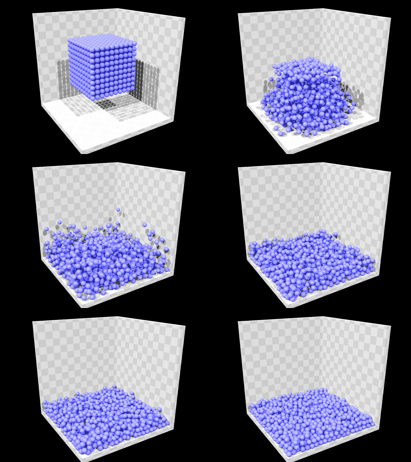
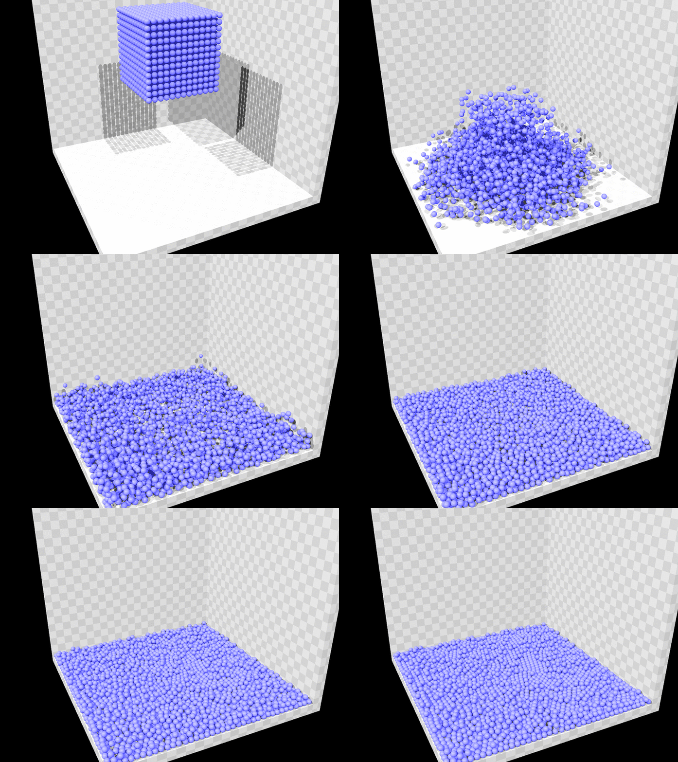
The simulations below shows a systems of 512, 1000 and 2917 particles
LATTICE-SPRING MODEL A more different set of systems can be approached with the LSM model, which is used to simulate the mechanical and elastic properties of certain materials, and also in medical imaging (see Echography simulation using the LSM).
LMS systems are formed by particles in lattices, joined to their neighbors by springs and dampers, and the equation of motion of the particles is given by the generalization of the classical mass-spring-damper system

For a particle i joined to N of their neighbors in this way, its equation of motion has the form

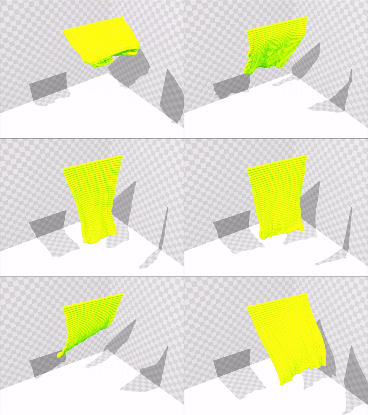
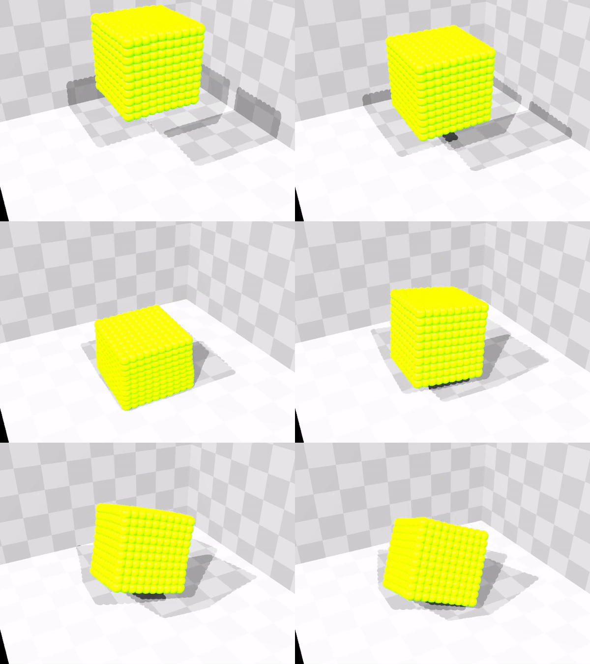
The systems below were simulated with this LSM equation by using 2D and 3D lattices, adding a gravitational force and using the boundary conditions of the hard spheres system.
All the systems shown above have the same code structure, that is, one uses a numerical method like Verlet’s to solve the equations of motion for a given potential or forces using certain boundary conditions. Many of the subroutines commonly used in this type of simulations are given in UAM’s “Computational methods in condensed matter physics” notes available at http://www.uam.es/personal_pdi/ciencias/evelasco/doctorado03-04/
More on Verlet algorithm, Molecular Dynamics and Monte Carlo simulations can be found in: Tao Pang (1997). “An introduction to computational physics”
LSM in medical imaging: C. Nastar and N. Ayache (1996). “Frequency-based Non-rigid Motion Analysis: Application for Four Dimensional Medical Imaging”. DOI: 10.1109/34.544076


Comentarios